Orbit Maintenance Model
This section explains the algorithm behind the fast but approximated orbit maintenance simulations (“Sam’s Simulator”).
The key idea is that one does not need to obtain all six parameters of the spacecraft during orbit propagation! Where a sufficiently accurate drag model is available, one really just needs the radial magnitude of the spacecraft in order to characterise the orbital energy loss due to the atmospheric density. This simplifies the number of calculations needed. In this section, the derivation of the decay model will be shared.
The goal of this exercise is to derive how the rate of change of a satellite’s radial distance relates to the drag forces at play. We begin with first principles - an expression on the orbit state energy - and find its derivative with respect to time and altitude.
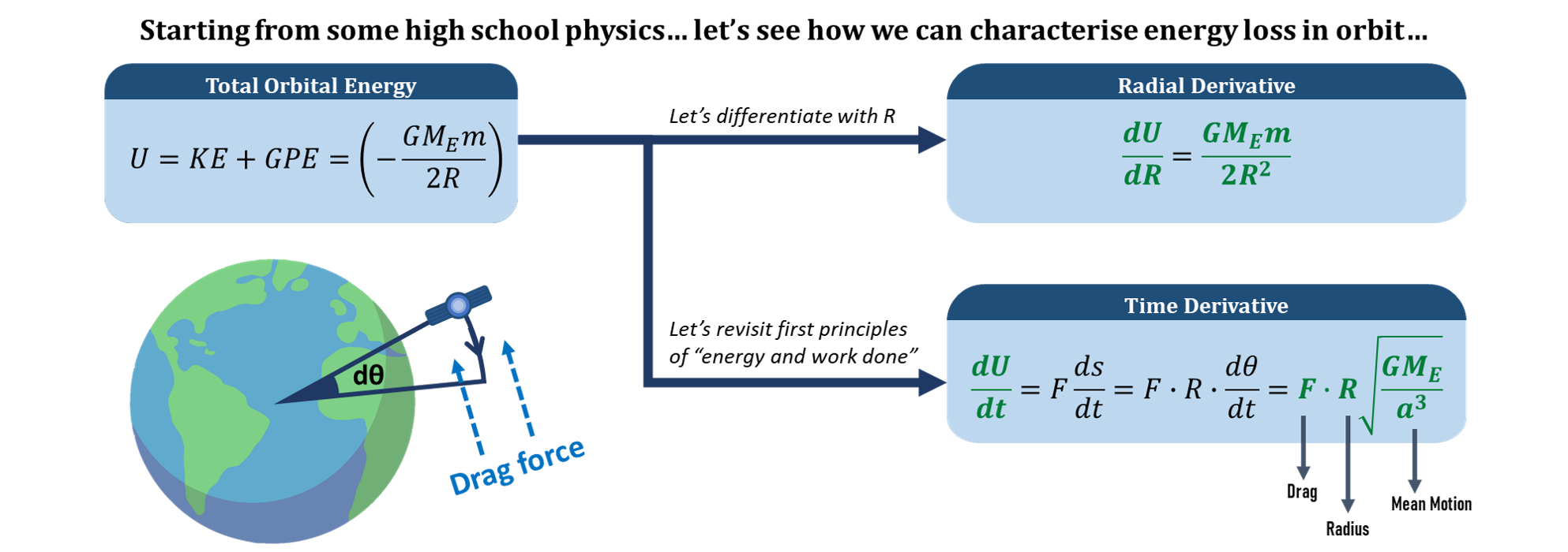
Figure 4.1 - Derivative of orbit state energy with respect to time and altitude.
The rate of change of work done by drag forces can be multiplied with the inverse of the altitude derivative of orbital energy, thereby removing the energy differential, dU, as the common term. Now, we have an expression for the rate of altitude change! We simply need to input the drag force F, and the radial distance of the satellite R.
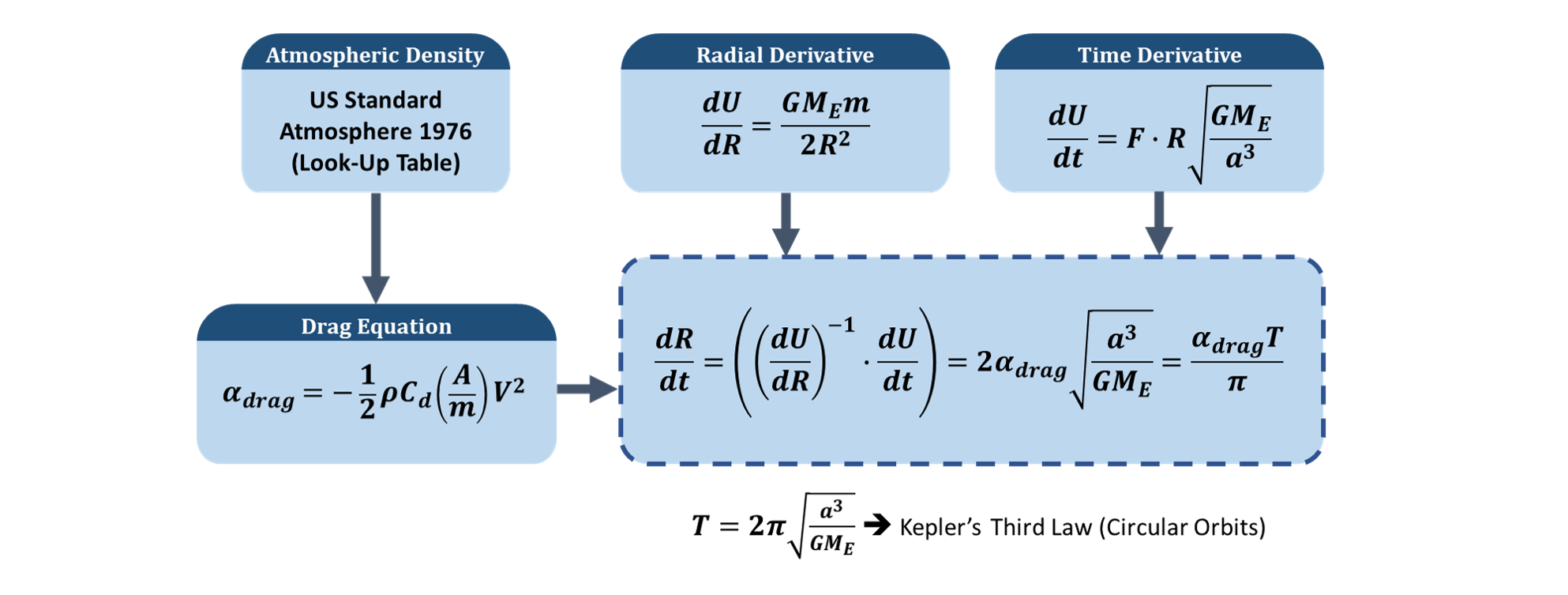
Figure 4.2 - Deriving the rate of change of the satellite altitude.
The radial distance R can be solved for through Kepler’s Equation in the Python file orbitm_func_kepler.py and using the input orbit parameters for a purely Keplerian orbit.
The drag force F, or equivalently the drag acceleration α, is computed via the standard drag equation, as a result of the satellite area-to-mass parameters (as set by the user), and the atmopsheric density value at radial distance R. The density is sourced from orbitm_func_atmos.py. This file is basically the U.S. Standard Atmosphere 1976, represented as a look-up table of coefficients for an exponential atmospheric model.
Simplifying the altitude decay rate model, we arrive at the elegant statement in 4.3:

Equation 4.3 - Decay rate = product of drag deceleration and Keplerian period, divided by Pi
This is powerful, because it proves that the rate at which the orbit decays can be solved in closed-form without any full orbit propagation of orbit states! This is the reason why orbit maintenance computations are extremely fast on ORBITM.
As the decay rate is also small, the total decay appears almost linear within the time frame of a single LEO orbital period (~95 minutes). Thus, a larger step size can also be used, without compromising too much on accuracy.
Consequently, the ORBITM program simply loops through the scenario time, and computes the decay in each time step until the spacecraft descends below the Maintenance Tolerance Band, which then triggers an orbit raise. This repeats until the end of the simulation.