ORBITM
![]()
![]()
By: Samuel Y. W. Low
![]()
![]()
ORBITM stands for the Orbit Maintenance and Propulsion Sizing Tool, and it is an open-source, easy-to-use, free-ware orbit maintenance simulator and propulsion sizing tool, for anyone with a Python 3 installation. The software comes with its own built-in orbit decay model and maintenance simulator, and it is also interface-able with AGI’s Systems Tool Kit (STK) as an alternative simulator.
The objective of ORBITM is to allow for a quick sizing of low Earth orbit (LEO) mission lifetimes, sized against propulsion units of the user’s choosing. The user may input into the UI their orbital parameters, spacecraft properties (mass, area, drag parameters etc), and the software will compute your desired ΔV necessary for the mission, track the altitude profile over time, and plot the thruster-fuel profile that satisfies the orbit maintenance needs of your mission.
Why was ORBITM created? In the New Space operating paradigm, the space engineering model no longer competes using the slow, sequential, and risk-intolerant development process. Agile development demands re-iteration of spacecraft designs quickly. Every iteration of a new spacecraft structure (for example, a change in choice of solar panels, or a new radar reflector type) changes the drag characteristics and mission life-time of LEO missions.
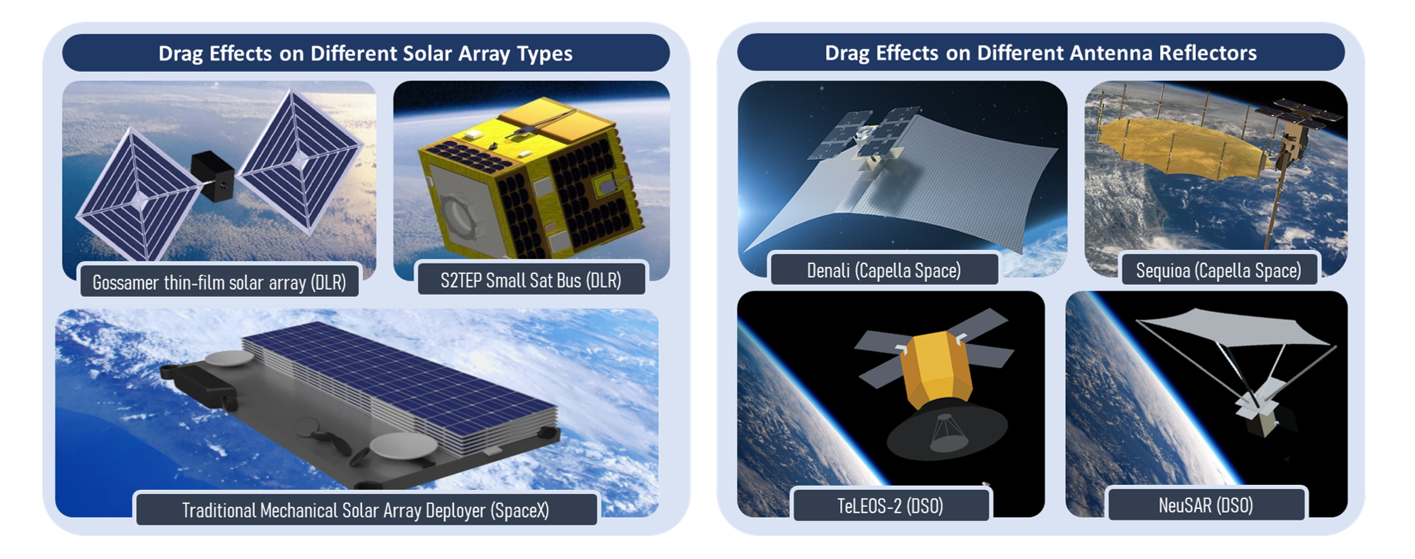
Figure 1.1 - Agile development demands that the mission planner can perform frequent mission life comparisons over rapidly changing iterations of spacecraft structures.
Traditional orbit maintenance simulations can be cumbersome and tedious to do on STK, GMAT, FreeFlyer, or even on your own code. Thus, ORBITM simplifies this entire drag-simulation process - in a fast and automated way that keeps up with rapidly changing iterations, without over-burdening the mission planner with repeated mission life-time simulations.
There are two modes of simulation available in ORBITM.
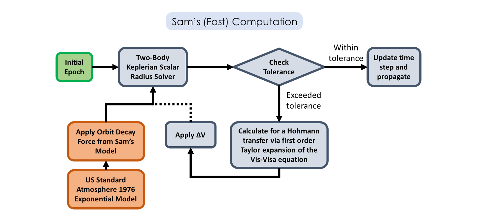
The first, is a fast-compute orbit decay and maintenance model considering primarily drag effects using the U.S. Standard Atmosphere 1976 model (Sam’s Simulator).
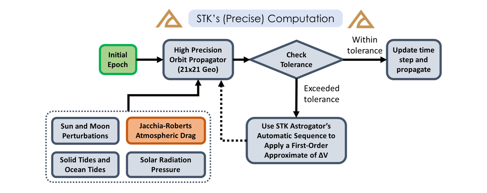
The second is a more accurately modelled but resource intensive mode that interfaces with and automates STK Astrogator to perform a high-precision orbit decay and maintenance simulation. The orbit model in STK uses a 21 by 21 (degree by order) geopotential, accounting also for radiation pressure and drag using a Jacchia-Roberts Atmospheric Density model.
However, in the second mode, you would need a valid STK Astrogator and STK Integration license installed with STK 10 or 11, for the interfacing to work.
Note
ORBITM was designed for low Earth orbits. Thus, the working range of altitudes, before loss of atmospheric density accuracies, should be bounded within 86 - 1,000 km.
1. Installation
First, find the ORBITM GitHub repository in this GitHub link, and download it. Alternatively, if you have Git installed, you can open Command Prompt or your Git Bash, enter the directory of your choice, and type:
git clone https://github.com/sammmlow/ORBITM.git
That’s it! No further setup is needed.
Note
Packages Required: numpy, matplotlib, tkinter, PIL, os, math, datetime, comtypes (for STK)
2. First Steps
ORBITM can be launched simply by running the Python file orbitm.py in the main directory (equivalent to the directory on the master branch on ORBITM’s GitHub). You should see a GUI that looks like the one below, pop up:
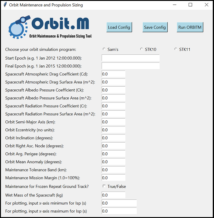
Figure 2.1 - ORBITM Graphical User Interface
As a first step, you can simply load the default input parameters by clicking “Load Config”. The parameters are actually saved in the config.txt file. Configuration parameters should be loaded through the GUI, and not manually updated through the config.txt file since then the software can’t check for string formatting errors (e.g. a negative drag coefficient that was typed into the config file manually and by accident would crash the program).
Warning
An orbit eccentricity of exactly zero is not allowed, to prevent potential divide-by-zero issues during calculations. For near-perfectly circular orbits, set an arbitrarily small eccentricity number (e.g., 0.00001).
Second, you can choose which lifetime and maintenance simulator you would like to use. By default, the native “Sam’s Simulator” will be selected. If STK is selected, remember that a valid STK license for STK Integration and STK Astrogator is required.
Third, proceed to set the remainder of your orbit and spacecraft parameters. These parameters are self-explanatory. Some parameters are specific to ORBITM and are defined below:
- Maintenance Tolerance Band
Threshold altitude that triggers an orbit raise (km).
- Maintenance Mission Margin
Multiplier applied to the mission’s life-time ΔV needs.
- Frozen Repeat Ground Track
Option to consider frozen repeat orbit maintenance.
Note
“Sam’s Simulator” mode uses the definition of the Maintenance Tolerance Band above in the Keplerian sense, or a pure ellipse in other words, on a purely spherical Earth. However, in STK-mode, due to oblateness of the Earth, and the presence of other perturbing forces, the Earth-centered altitude often oscillates with time, even for a “circular orbit”.
In order to prevent triggering a manoeuvre on the wrong rising or falling edge of the altitude profile, the STK mode triggers manoeuvres based on the Kozai-Izsak Mean Semi-Major Axis rather than the nominal altitude + Earth radius. It is acknowledged that this changes the definition for the “threshold altitude”, especially for highly elliptical orbits running in STK.
If the option for a Frozen Repeat Ground Track was selected, then the orbit raise will happen from the threshold below its initial altitude to a positive threshold above the initial altitude, and the thrusts will be done in perigee-apogee pairs. This minimises secular perturbations to the orbit mean eccentricity and the orbit nodal period. For example, if the Frozen Repeat Ground Track option was selected, with an initial altitude of 500km, and a threshold of 5km, the orbit raise will be triggered at 495km, and raised to 505km in two thrust pairs. Else, in the non-frozen repeat orbit maintenance case, the orbit raise will be triggered at 495km, and raised back to the original 500km.
Finally, before running the simulation (Run ORBITM), check the “thruster_shortlist.txt” file on the main ORBITM directory, and add thruster specifications that you wish to size your missions against. Some thrusters are written inside this shortlist as an example. The purpose of this shortlist is to provide the program with the thruster specifications, so that the mission planner can graphically compare its Isp and fuel capacity to the suitability of the mission (as an output of the program).
Now, you can run ORBITM. If you are a licensed STK user and you would like to use ORBITM to automate an orbit maintenance simulation in STK for you, make sure there are no running instances of STK before you run ORBITM in the STK 10 or 11 mode.
Note
“Sam’s Simulator” does not include albedo and radiation effects, thus tuning these parameters will have no effect in the “Sam’s” mode. However, they are considered when using STK.
3. Interpreting Results
To interpret the results, we explore three example scenarios for ORBITM - each is a circular orbit at 63.4 degrees inclination, at 450km, 500km, and 550km mean altitude respectively.
The plots in blue correspond to “Sam’s Simulator”. The plots in orange correspond to using STK 10 Astrogator, with a high precision orbit propagator, and it uses Astrogator’s Automatic Sequences feature to boost the orbit up whenever the altitude of the spacecraft crosses the minimum of the maintenance tolerance band. In both orbit maintenance modes, the ΔV values were computed using a first order Taylor expansion to the Vis-Visa equation.
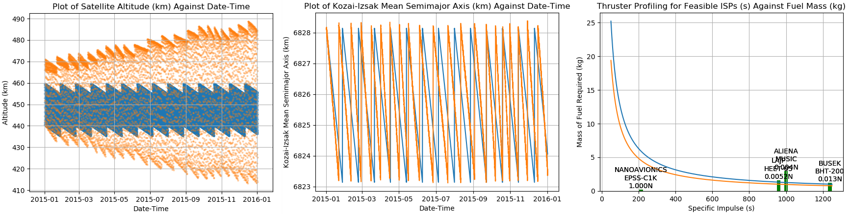
Figure 3.1 - Circular orbit at 450km; tolerance band of 5km
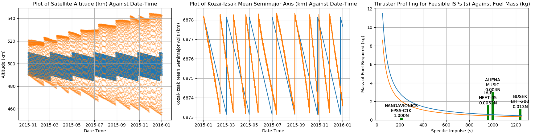
Figure 3.2 - Circular orbit at 500km; tolerance band of 5km
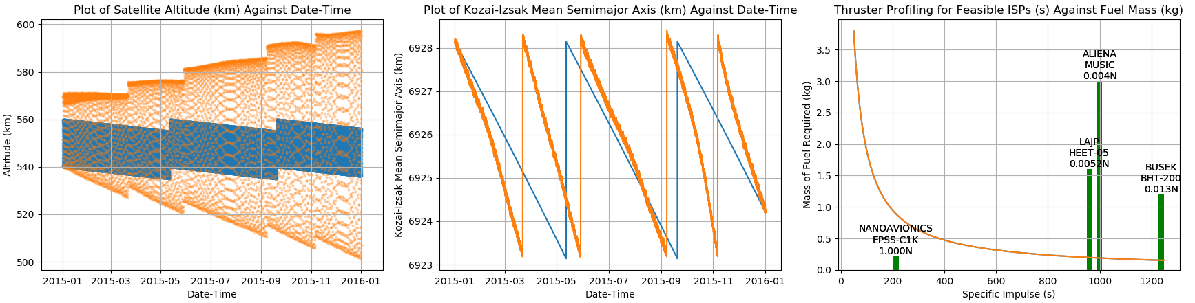
Figure 3.3 - Circular orbit at 550km; tolerance band of 5km
The plot most relevant to mission planning that you would need is the third one from the left - the profile of the mission lifetime (in terms of total ΔV requirements) against the thruster specifications (bar charts). The height of the bar chart can be compared against the desired fuel mass needed, at the thruster’s specific impulse values (Isp, units in seconds). In other words, for each thruster’s Isp value, if the height of the bar chart (which represents the max fuel mass for that thruster, at that Isp) exceeds the fuel mass requirements of your mission at that particular Isp, then that thruster can satisfy your mission lifetime requirements.
Note
You can scale your fuel mass requirements in the line plots (in both blue and orange plots) by increasing the Maintenance Mission Margin parameter in the GUI (see Figure 2.1). A value of 1.0 implies that the program will compute the fuel mass and ΔV equivalently needed to counter 100% of the drag effects you encounter. If you would like to have a margin of 3x amount of fuel, then input 3.0 as your mission margin.
The program will also output a time-schedule for orbit maintenance in the main directory of ORBITM, as a text file “deltaV.txt”. This file gives you the time stamps of when each thrust should occur, which is primarily dependent on the decay computation (drag effects) and your chosen tolerance band (i.e. how far do you descend before you fire your thrusters).
4. Fast Orbit Maintenance
This section explains the algorithm behind the fast but approximated orbit maintenance simulations (“Sam’s Simulator”).
The key idea is that one does not need to obtain all six parameters of the spacecraft during orbit propagation! Where a sufficiently accurate drag model is available, one really just needs the radial magnitude of the spacecraft in order to characterise the orbital energy loss due to the atmospheric density. This simplifies the number of calculations needed. In this section, the derivation of the decay model will be shared.
The goal of this exercise is to derive how the rate of change of a satellite’s radial distance relates to the drag forces at play. We begin with first principles - an expression on the orbit state energy - and find its derivative with respect to time and altitude.
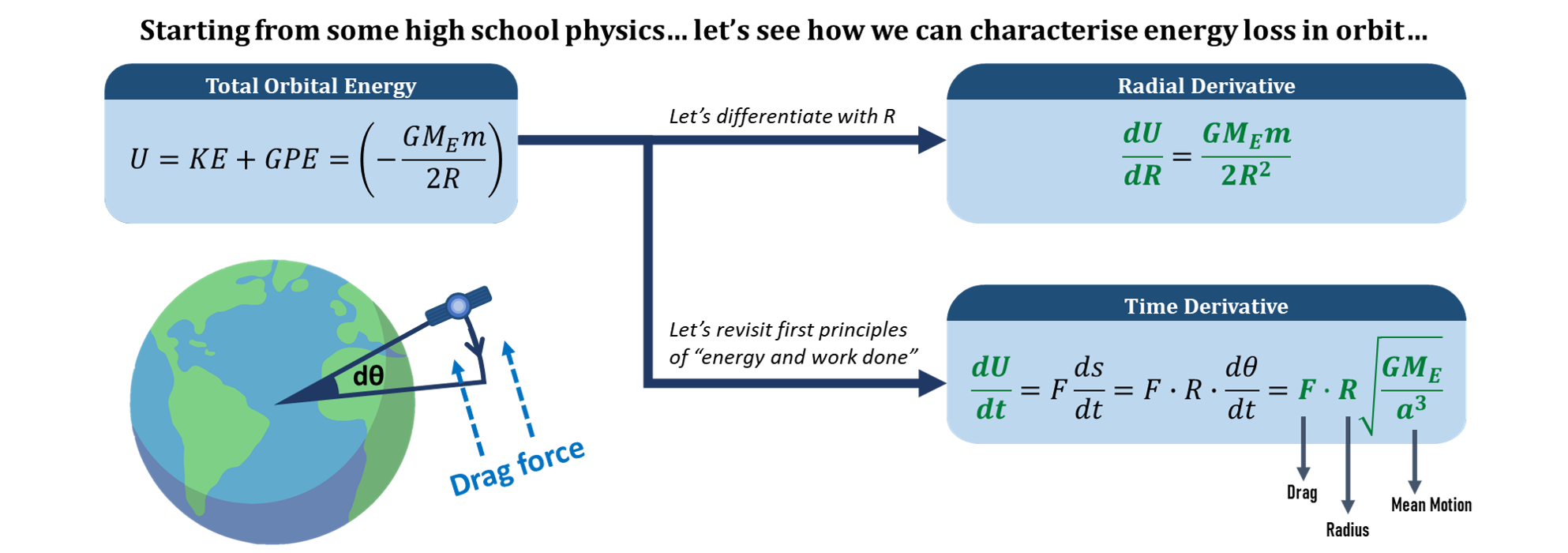
Figure 4.1 - Derivative of orbit state energy with respect to time and altitude.
The rate of change of work done by drag forces can be multiplied with the inverse of the altitude derivative of orbital energy, thereby removing the energy differential, dU, as the common term. Now, we have an expression for the rate of altitude change! We simply need to input the drag force F, and the radial distance of the satellite R.
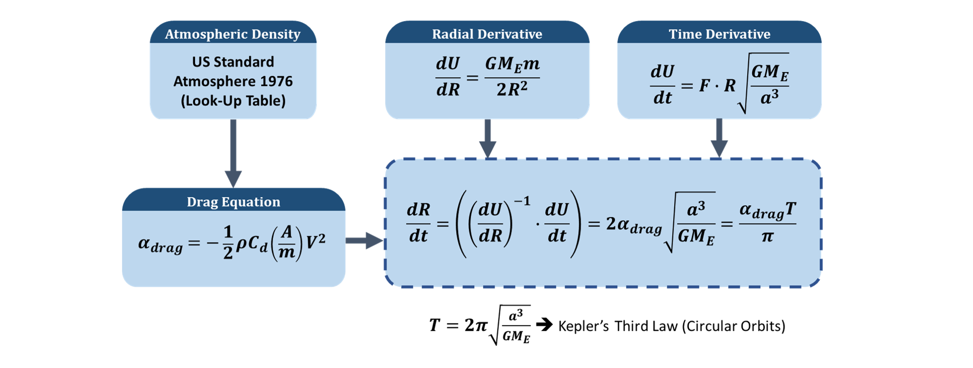
Figure 4.2 - Deriving the rate of change of the satellite altitude.
The radial distance R can be solved for through Kepler’s Equation in the Python file orbitm_func_kepler.py and using the input orbit parameters for a purely Keplerian orbit.
The drag force F, or equivalently the drag acceleration α, is computed via the standard drag equation, as a result of the satellite area-to-mass parameters (as set by the user), and the atmopsheric density value at radial distance R. The density is sourced from orbitm_func_atmos.py. This file is basically the U.S. Standard Atmosphere 1976, represented as a look-up table of coefficients for an exponential atmospheric model.
Simplifying the altitude decay rate model, we arrive at the elegant statement in 4.3:

Equation 4.3 - Decay rate = product of drag deceleration and Keplerian period, divided by Pi
This is powerful, because it proves that the rate at which the orbit decays can be solved in closed-form without any full orbit propagation of orbit states! This is the reason why orbit maintenance computations are extremely fast on ORBITM.
As the decay rate is also small, the total decay appears almost linear within the time frame of a single LEO orbital period (~95 minutes). Thus, a larger step size can also be used, without compromising too much on accuracy.
Consequently, the ORBITM program simply loops through the scenario time, and computes the decay in each time step until the spacecraft descends below the Maintenance Tolerance Band, which then triggers an orbit raise. This repeats until the end of the simulation.
5. Contact and Reference
If ORBITM has made your life somewhat easier, please do cite the work behind it!
For bugs, raise the issues in the GitHub repository.
For collaborations, reach out to me: sammmlow@gmail.com (Samuel Y. W. Low)
![]()
![]()
The project is licensed under the MIT license.